Implementation and Analysis of Sorting
- Course: Data Structures
- StudentID: 2466044
- Author: LEE SIEUN
- Date: 2025-11-18
- Repository(public): https://github.com/sihyes/2025-Data-Structures/tree/main/07-Sorting
#0. Assignment Goals
The original question number 2 is written in hand-written-technical-report. This report deals only with programming assignments.
1.Implement a stable version of selection sort.
- Analyze the stable sorting result for the given input.
- Modify the traditional (unstable) selection sort to produce stable output.
2. Analyze the pseudo code of the Partition algorithm (p36). (handwritten)
- Explain its logic and derive its time complexity.
3. Implement radix sort using counting sort.
- Generate 1000 random 24-bit integers.
- Split each integer into four 6-bit segments.
- Sort from least significant digit to most significant using counting sort.
#1. Introduction(Theoretical Background, Logic)
데이터를 정렬하는 방법에는 다양한 알고리즘이 존재하며, 알고리즘마다 연산 횟수가 다르므로 시간복잡도도 다르다. 정렬 알고리즘을 선택할 때는 구현 난이도, 연산 효율, 안정성(stability) 등을 고려해야 한다.
Stable vs Unstable Sorting
- Stable (안정적 정렬): 동일한 값의 데이터가 정렬 후에도 원래 순서를 유지하는 경우
- Unstable (불안정적 정렬): 동일한 값의 데이터 순서가 정렬 과정에서 바뀌는 경우
예시: [5, 3a, 1, 3b] → stable 정렬: [1, 3a, 3b, 5], unstable 정렬: [1, 3b, 3a, 5]
분류
- 간단하지만 비효율적인 알고리즘: Insertion Sort, Selection Sort, Bubble Sort
- 복잡하지만 효율적인 알고리즘: Quick Sort, Heap Sort, Merge Sort, Radix Sort
- 메모리 기준:
- Internal sort: 대부분의 데이터가 메인 메모리에 존재
- External sort: 데이터 대부분이 외부 저장장치에 존재, 일부만 메모리에 존재
1.1 다양한 정렬 알고리즘 요약
알고리즘 핵심 아이디어 안정성 시간복잡도 (평균)
| Selection Sort | 오른쪽 리스트에서 최소값 탐색 후 왼쪽과 스왑 | 불안정 | O(n²) |
| Insertion Sort | 정렬된 왼쪽 리스트에 적절한 위치에 삽입 | 안정 | O(n²) |
| Bubble Sort | 인접한 요소 비교 후 스왑 | 안정 | O(n²) |
| Merge Sort | 분할 정복, 정렬 후 병합 | 안정 | O(n log n) |
| Quick Sort | Pivot 기준 좌우 분할, 재귀적 정렬 | 불안정 | O(n log n) |
| Counting Sort | 값의 개수를 세어 직접 위치에 배치 | 안정 | O(n + k) |
| Radix Sort | 자릿수별로 Counting Sort 반복 | 안정 | O(d*(n+k)), d: 자릿수 |
| Shell Sort | 일정 간격으로 부분 정렬 후 간격 줄이기 | 불안정 | O(n log² n) (최악: O(n²)) |
핵심: Stable 여부, 연산 방식, 시간복잡도를 보고 적절한 정렬 알고리즘을 선택 가능.
Data can be sorted using various algorithms, each with different computational costs, resulting in different time complexities. When choosing a sorting algorithm, it is important to consider implementation difficulty, efficiency, and stability.
Stable vs Unstable Sorting
- Stable: Identical elements retain their original relative order after sorting.
- Unstable: Identical elements may change their original relative order.
Example: [5, 3a, 1, 3b] → stable sort: [1, 3a, 3b, 5], unstable sort: [1, 3b, 3a, 5]
Classification
- Simple but inefficient algorithms: Insertion Sort, Selection Sort, Bubble Sort
- Complex but efficient algorithms: Quick Sort, Heap Sort, Merge Sort, Radix Sort
- Memory-based sorting:
- Internal sort: most data resides in main memory
- External sort: most data resides in external storage, only part in main memory
1.1 Summary of Various Sorting Algorithms
| Algorithm | Key Idea | Stability | Time Complexity (Average) |
| Selection Sort | Find the minimum in the right sublist and swap to left | Unstable | O(n²) |
| Insertion Sort | Insert current element into the correct position in sorted left | Stable | O(n²) |
| Bubble Sort | Compare and swap adjacent elements | Stable | O(n²) |
| Merge Sort | Divide and conquer, merge sorted sublists | Stable | O(n log n) |
| Quick Sort | Partition around a pivot recursively | Unstable | O(n log n) |
| Counting Sort | Count occurrences and place elements directly | Stable | O(n + k) |
| Radix Sort | Apply Counting Sort digit by digit | Stable | O(d*(n+k)), d: number of digits |
| Shell Sort | Sort sublists with decreasing gap | Unstable | O(n log² n) (Worst: O(n²)) |
>> Key points: Choose sorting algorithm based on stability, operational logic, and time complexity.
주어진 데이터를 정렬하는 방법에는 다양한 방법이있다. 정렬에 다양한 방법이 존재함에 따라, 각 방법별로 연산이 수행되는 횟수가 다르므로 시간복잡도 또한 다르다.
각 방법의 구현 난이도, 핵심 아이디어, 시간복잡도를 비교해보자.
여기에서 Stability이라는 단어가 나온다. stable이란 무엇인가? 같은 데이터가 있을때, 해당 데이터의 순서가 유지되는가를 묻는 상태이다.
예를들어 sort [5,3,1,3]이라는 배열을 정렬한다고 가정하자. 3이라는 데이터가 두 번 나오므로, 중복이다. 이때 각각의 데이터는 값은 같지만 메모리상에는 다른 메모리에저장되므로, 앞에있는 데이터를 a, 뒤에있는 데이터를 b라고 가정하자.
[5 ,3a, 1, 3b]
정렬 연산 후
[1, 3a, 3b, 5]
이와 같이 동일데이터라도, 기존의 순서를 유지하며 정렬되는것을 stable한 sorting이라고 부른다.
[1,3b,3a,5] 이처럼 같은 데이터에 대해 순서가 바뀌어 정렬된다면 unstable이라고 이야기한다.
수업에서 다룬 자료구조들을 정리해보자.
- Simple but inefficient algorithms:
- Insert sort, selection sort, bubble sort - Complex but efficient algorithms
- Quick sort, heap sort, merge sort, radix sort - Internal sort
- sort a set of data that stored in main memory - External sort
- Sort a set of data whem moost of the data is stored in the external storagme device and only a part of the data is stored in the main memory.
#1.1 various Sorting
Selection Sort
| sort name | key idea |
| Selection Sort (비교 후 선택) | from left(sorted) to right (unordered data) 1. search a minimum value in the rightside. 2. swap A[0] with A[minimum_index] 3. leftlist size ++, rightlistsize -- (= then, iterate 1,2 with A[1] with its rightlist until rightlist empty) |
| Insertion Sort (선택 후 비교해서 정렬) | from left(sorted) to right (unordered data) 1. Select A[0] (ordered) 2. Select A[1] ... find appropriate index in left list(ordered list) 3, insert A[1] into that index. iterate until rightlist is empty |
| Bubble Sort(인접한 데이터 비교 및 스왑 n^2 루프) | |
| Merge Sort (중간기점으로 나눠서하는 분할정복) | |
| Quick Sort (피봇 설정해서 왼쪽오른쪽 한번에 나중에 원위치) | |
| Counting sort | |
| Radix sort | |
| 번외) Shell Sort |
#2. Problem Definition
1.(Programming: 35 points) The selection sort is known to produce unstable sorting results. The attached code is a simple instance of unstable sorting results.
First, explain the stable sorting result of the following input, and then implement ‘selection_sort_stable’ that produces the stable sorting result.
Note) It is not mandatory to follow the data structure used in the attached code. Feel free to revise it, if needed.
typedef struct data{
		int * id;
        int * score;
} data;

int data_id[] = { 1, 2, 3, 4, 5, 6, 7, 8 };
int data_score[] = { 30 , 25 , 10 , 20 , 80 , 30 , 25 , 10 };
2. (Hand-written homework: 5 points)
Analyze and explain the pseudo code and its time complexity of ‘Partition’ in p36 (‘Another Solution for Partition’) of ‘DS-Lec09-Sorting’.
3. (Programming: 60 points)
The radix sort was implemented using queue in p51 of the lecture note. Revise this code by using the counting sort in p42 instead of the queue.
Step 1) Generate the input data to be sorted randomly.
# of input data: 1000 integers (data range: 0 ~224-1, i.e., 24-bit positive integer)
Step 2) Divide each data into 4 segments, i.e., each segment consists of 6 bits.
Step 3) Sort values at each digit from LSD to MSD.
Namely, in p47 of ‘DS-Lec09-Sorting.pdf’, n=1000, b=24, r=6, b/r=4 (# of digits)
Note)
- Consider what the data structure is needed to implement the radix sort using the counting sort.
- It is recommended NOT to use expensive arithmetic operators (division / and remainder operator %).
RadixSort(A, d)
	for i=1 to d
		Counting Sort(A) on digit i
#3. Algorithm and Data Structure
For Problem 1, we implemented Selection Sort, which is a simple comparison-based sorting algorithm. Although traditional selection sort is unstable, we modified it to produce a stable sorting result. The core idea is to repeatedly select the minimum element from the unsorted portion of the array and insert it into its correct position in the sorted portion, while preserving the relative order of equal elements. In our implementation, we used a struct data type to store paired id and score values, ensuring that stable sorting could be achieved based on score while keeping id as a tie-breaker for identical scores.
For Problem 3, we implemented Radix Sort using Counting Sort as the subroutine for digit-level sorting. Traditionally, the lecture note used queues to manage elements at each digit, but in our implementation, Counting Sort was used to efficiently count occurrences and determine the position of elements at each digit. The input data consists of 1000 randomly generated 24-bit integers, divided into 4 segments of 6 bits each. Sorting is performed from the least significant digit (LSD) to the most significant digit (MSD). This approach preserves the stability of the sorting at each digit, which is crucial for Radix Sort to work correctly
#4. Implementation Results and Analysis
4.1 Implementation of stable sorting
4.1.1 First, explain the stable sorting result of the following input.
Here are some data which has same value(30,25,10). then what is stable sorting? the order before sorting and after sorting is equal. let first 30 as 30a, second 30 as 30b,,, then the sorted data should be 30a 30b (Not 30b 30a).
here is the stable version of data. then how we can implement it?
selection sort is sorting from leftmost to rightmost by switching index. left = sorted, right - unordered data
Procedure
1. Select the minimum value in the right list and exchange it with the first number in the right list.
2. Increase the left list size
3. Decrease the right list size Iterate 1-3 until the right list is empty
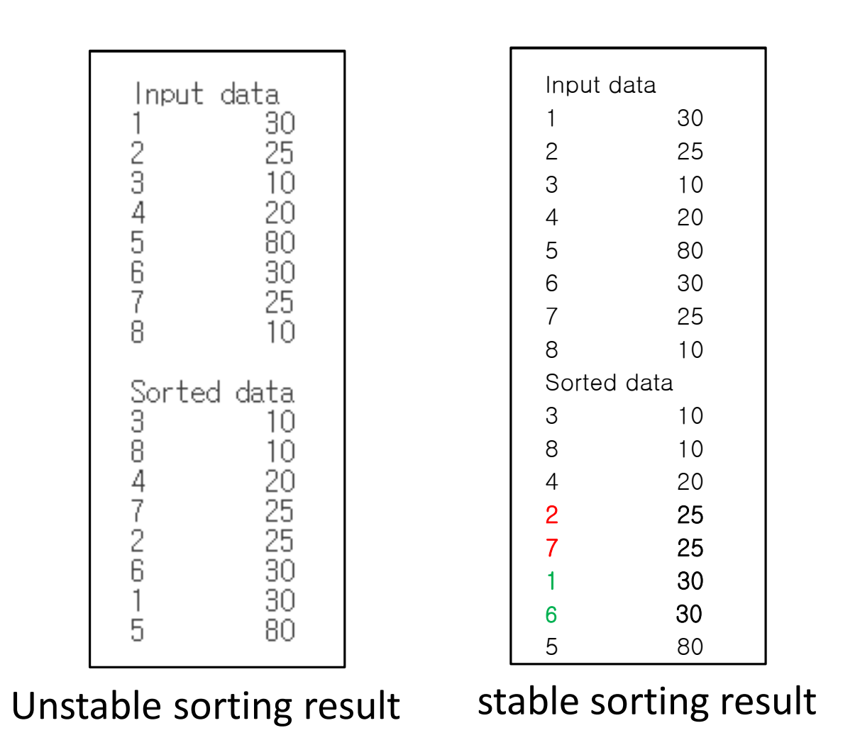
4.1.2 Second, explain the stable sorting result of the following input.
Below are the actual implementation results. You can see that it's output normally (id was well aligned in ascending order)


void selection_sort_stable(data *list, int n)
{
    //기본적으로 비슷하다. 그러나, 찾아서 스왑하는게 아닌, 찾아서 '삽입'식으로 바꿔보자.
    int i, j, least;
    int tmpid, tmpscore;
    for (i = 0; i < n - 1; i++) {
        least = i;
        for (j = i + 1; j<n; j++)
            if (list->score[j]<list->score[least]) least = j;
        // 기존 배열의 인덱스를 한칸씩 뒤로 밀고, 찾은 최솟값을 맨앞에 넣어주자.,
        // 최소값 임시 저장
        tmpid = list->id[least];
        tmpscore = list->score[least];

        for (j=least; j>i;j--) {
            list->score[j]=list->score[j-1];
            list->id[j]=list->id[j-1];
        }
        list->id[i]=tmpid;
        list->score[i]=tmpscore;
    }
}
#4.2 Implementation of Radix Sorting using counting sort
#4.2.1 data structures
A Radix Sort algorithm was implemented to sort 24-bit integers.
Each integer is divided into four 6-bit segments.
Starting from the least significant bits (LSD), Counting Sort is repeatedly applied for each 6-bit segment, resulting in a fully sorted 24-bit integer array.
Correctness was verified by comparing the output against the standard C library’s `qsort`.
#4.2.2 Key concept Explanations
Generating 24bit numbers
Only 24 bits are required, so the result of `rand()` was masked:
This guarantees numbers strictly in the range: $ 0 to (2^24 - 1)$
rand() & 0b111111111111111111111111
for operate with only 6 bits...
typedef struct data {
    unsigned int value;
    unsigned int seg;
} data;
이렇게 데이터를 설정해놓고, 원래의 데이터와 세그먼트를 저장하는 `data`를 만들었다.
Segment Extraction method : Each 6-bit segment is extracted using!
(value >> (6 * d)) & 0b111111here d runs from 0 to 3:
- `d = 0` → lowest 6 bits
- `d = 1` → next 6 bits
- `d = 2` → next 6 bits
- `d = 3` → highest 6 bits
This is the core of the LSD-to-MSD Radix Sort process.
Role of Counting Sort
Counting Sort performs stable sorting based solely on the current 6-bit segment.
Since each segment ranges from 0 to 63, a count array of size 64 is required.
A Counting Sort pass consists of:
- Histogram (frequency count)
- Prefix sum (cumulative count)
- Stable output construction (fill from the back)
Stability is essential because Radix Sort requires the original relative order of equal keys to be preserved.
This is why elements must be inserted starting from the last index.
Why Pointer Swapping in Radix Sort Is Important
This was the most confusing part during development.
The initial implementation used:
counting_sort(A, tmp, n);
for (i = 0; i < n; i++) A[i] = tmp[i];
This unnecessarily copies the entire array every pass.
However, after Counting Sort finishes, `tmp` already contains the newly sorted order for the current segment.
The next pass should use this sorted result as its new input array.
Rather than copying, simply swap the pointers:
data *swap = A;
A = tmp;
tmp = swap;
- The actual memory content stays the same.
- Only the “labels” A and tmp exchange roles.
- The next pass reads from the freshly sorted tmp.
Then, finally `O(n) array copy → O(1) pointer swap`. This provides a major efficiency improvement.
Copy input → A

For d = 0 to 3:
    Extract segment from A[i].value
    counting_sort(A → tmp)
    swap(A, tmp)

After final pass:
    Copy A back to original array (if needed)

Compare with qsort to validate correctness
Here is the final code.
Making the correct answer array created a comparison group with the help of AI.
//
// Created by sinil on 2025-11-14.
//

#include "stdlib.h"
#include "stdio.h"
#include "string.h"
#include <time.h>


typedef struct data {
    unsigned int value; // (원래 값)
    unsigned int seg; // 현재 sorting segment 값 (0~63)
} data;

unsigned int random24() {
    // 24비트 랜덤 숫자를 생성합니다.
    return (unsigned int) (rand() & 0b111111111111111111111111); // 마스크 길이를 24개로.
}

unsigned int getSeg(unsigned int value, int d) {
    return (value >> (6 * d)) & 0b111111; // d가 0,1,2,3 으로가면서6비트씩 읽어나가요)
}

void counting_sort(data *A, data *output, int n) {
    int count[64] = {0};

    //1. 히스토그램
    for (int i = 0; i < n; i++) {
        count[A[i].seg] += 1; // 히스토그램, 즉 각 세그먼트별 개수를 모아요
    }

    //2. 누적합
    for (int i = 1; i < 64; i++) {
        count[i] += count[i - 1];
    }

    // 3. stable sort (뒤에서부터!)
    for (int i = n-1; i >=0; i--) {
        //각 세그먼트를 기존 배열에 다시 위치를 재조정해서 배치해보아요. seg기준으로!
        int s = A[i].seg;
        output[count[s]-1]=A[i];
        count[s]--;
    }
}

void RadixSort(unsigned int * array, int n) {
    //수의 배열과, 분할할 비트수를 받아옵니다.
    data *A = (data *)malloc(sizeof(data) * n);
    data *tmp = (data *)malloc(sizeof(data) * n);

    if (!A || !tmp) {
        printf("Memory allocation failed!\n");
        exit(1);
    }

    //원본 값을 복사
    for (int i=0; i<n; i++) {
        A[i].value = array[i];
    }

    // LSD segment부터 네번 처리하면된다.
    for (int s = 0; s < 4; s++) {
        //segment 설정
        for (int i=0; i<n; i++) {
            A[i].seg = getSeg(A[i].value,s); // segment를 받아온다. 원래값주고 몇번째 세그먼트(몇번 shift할건지)
        }

        counting_sort(A,tmp,n);

        data *swap = A; // 포인터를 바꾼다. 즉, 특정 변수명에 담긴 주소를 스윗치~
        A = tmp;
        tmp = swap;
    }
    for (int i=0; i<n; i++) {
        array[i]=A[i].value; // 값들을 다시저장한다.
    }
}
int cmp(const void *a, const void *b) {
    unsigned int x = *(unsigned int *)a;
    unsigned int y = *(unsigned int *)b;

    if (x < y) return -1;
    if (x > y) return 1;
    return 0;
}

int main() {
    int i;
    int n = 1000;
    srand(time(NULL)); // 시드 초기화

    unsigned int *list = (unsigned int *)malloc(sizeof(unsigned int) * n);
    unsigned int *correct = (unsigned int *)malloc(sizeof(unsigned int) * n);

    if (!list || !correct) {
        printf("Memory allocation failed!\n");
        return 1;
    }

    //generate input data using random numbers (0~2^24 - 1)
    for (i = 0; i < n; i++) {
        list[i] = random24();
    }

    // 정답배열 만들기
    memcpy(correct, list, sizeof(unsigned int) * n);
    qsort(correct, n, sizeof(unsigned int), cmp);

    RadixSort(list, n);

    // 둘을 비교 시스템이 해준 정렬vsRadix Sort
    for (i=0; i<n; i++){
        if(correct[i] != list[i]) {
            printf("Mismatch at %d!\n", i);
            return 0;
        }
    }
    printf("Correct!\n");

    free(list);
    free(correct);

    //24비트의 양수를, 4개의 segment로 쪼갭니다. 각 세그먼트는 6비트로 이루어집니다.
    //24비트->6비트*4로 나눈 것 중, 각각의 세그먼트에 대해 6비트의 묶음들끼리 정렬을 시킵니다.
    //LSD(일의자리 숫자부터) 정렬을 해나갑니다.
    //✅ 1. 비트 쉬프트 연산자란?
    //<<    왼쪽 쉬프트 (비트를 왼쪽으로 밀기), x << n x를 왼쪽으로 n비트 이동 오른쪽을 0으로 채웁니다.
    //>>    오른쪽 쉬프트 (비트를 오른쪽으로 밀기)
    // 비트를 쪼갠다. (값 >> 이동량) & 마스크
    // 우리의 경우 6비트를 이용하므로 6자리, 111111을 이용한다. 0011 1111 ,, 16진수로 나타내자면 0x3F
    // 처음 6비트| 값 & 0x3F
    // 다음 6비트 ( 값 >> 6 ) 0x3F
    // 세그먼트에 따라서 순차적으로 정렬 한다!
    // n=1000, b=24, r=6, b/r=4 (# of digits)
    // RadixSort(A, d)
    //     for i=1 to d
    //         Counting Sort(A) on digit i


    //카운팅 소트를 하려면 그럼, 리스트가 4개 필요하고, 임시 리스트(누적합사용, 최종 리스트)가 있어야하는가요?
    // >> 아니다. 원본배열 -> 하위6비트 정렬 -> 그다음 6비트 -> 그다음 -> 마지막 상위 6비트 정렬 -> 최종적으로 정렬완료!
    // 원본 배열과, 아웃풋 배열만 있으면된다!


    return 0;
}
내 처음 구현...은
//
// Created by sinil on 2025-11-14.
//

#include "stdlib.h"
#include "stdio.h"
#include "string.h"
#include <time.h>


typedef struct data {
    unsigned int value; // (원래 값)
    unsigned int seg; // 현재 sorting segment 값 (0~63)
} data;

unsigned int random24() {
    // 24비트 랜덤 숫자를 생성합니다.
    return (unsigned int) (rand() & 0b111111111111111111111111); // 마스크 길이를 24개로.
}

unsigned int getSeg(unsigned int value, int d) {
    return (value >> (6 * d)) & 0b111111; // d가 0,1,2,3 으로가면서6비트씩 읽어나가요)
}

void counting_sort(data *A, data *output, int n) {
    int count[64] = {0};

    //1. 히스토그램
    for (int i = 0; i < n; i++) {
        count[A[i].seg] += 1; // 히스토그램, 즉 각 세그먼트별 개수를 모아요
    }

    //2. 누적합
    for (int i = 1; i < 64; i++) {
        count[i] += count[i - 1];
    }

    // 3. stable sort (뒤에서부터!)
    for (int i = n-1; i >=0; i--) {
        //각 세그먼트를 기존 배열에 다시 위치를 재조정해서 배치해보아요. seg기준으로!
        int s = A[i].seg;
        output[count[s]-1]=A[i];
        count[s]--;
    }
}

void RadixSort(unsigned int * array, int n) {
    //수의 배열과, 분할할 비트수를 받아옵니다.

    data A[n], tmp[n];
    //원본 값을 복사
    for (int i=0; i<n; i++) {
        A[i].value = array[i];
    }

    // LSD segment부터 네번 처리하면된다.
    for (int s = 0; s < 4; s++) {
        //segment 설정
        for (int i=0; i<n; i++) {
            A[i].seg = getSeg(A[i].value,s); // segment를 받아온다. 원래값주고 몇번째 세그먼트(몇번 shift할건지)
        }

        counting_sort(A,tmp,n);

        for (int i=0;i<n;i++) {
            A[i]=tmp[i]; // 다시 원본배열을 덮어씌운다.
        }
    }
    for (int i=0; i<n; i++) {
        array[i]=A[i].value; // 값들을 다시저장한다.
    }
}
int cmp(const void *a, const void *b) {
    unsigned int x = *(unsigned int *)a;
    unsigned int y = *(unsigned int *)b;

    if (x < y) return -1;
    if (x > y) return 1;
    return 0;
}

int main() {
    int i;
    int n = 1000;
    srand(time(NULL)); // 시드 초기화
    unsigned int list[n];

    //generate input data using random numbers (0~2^24 - 1)
    for (i = 0; i < n; i++) {
        list[i] = random24();
    }

    // 정답배열 만들기
    unsigned int correct[n];
    memcpy(correct, list, sizeof(list));
    qsort(correct, n, sizeof(unsigned int), cmp);

    RadixSort(list, n);

    // 둘을 비교 시스템이 해준 정렬vsRadix Sort
    for (i=0; i<n; i++){
        if(correct[i] != list[i]) {
            printf("Mismatch at %d!\n", i);
            return 0;
        }
    }
    printf("Correct!\n");

    //24비트의 양수를, 4개의 segment로 쪼갭니다. 각 세그먼트는 6비트로 이루어집니다.
    //24비트->6비트*4로 나눈 것 중, 각각의 세그먼트에 대해 6비트의 묶음들끼리 정렬을 시킵니다.
    //LSD(일의자리 숫자부터) 정렬을 해나갑니다.
    //✅ 1. 비트 쉬프트 연산자란?
    //<<	왼쪽 쉬프트 (비트를 왼쪽으로 밀기), x << n x를 왼쪽으로 n비트 이동 오른쪽을 0으로 채웁니다.
    //>>	오른쪽 쉬프트 (비트를 오른쪽으로 밀기)
    // 비트를 쪼갠다. (값 >> 이동량) & 마스크
    // 우리의 경우 6비트를 이용하므로 6자리, 111111을 이용한다. 0011 1111 ,, 16진수로 나타내자면 0x3F
    // 처음 6비트| 값 & 0x3F
    // 다음 6비트 ( 값 >> 6 ) 0x3F
    // 세그먼트에 따라서 순차적으로 정렬 한다!
    // n=1000, b=24, r=6, b/r=4 (# of digits)
    // RadixSort(A, d)
    //     for i=1 to d
    //         Counting Sort(A) on digit i


    //카운팅 소트를 하려면 그럼, 리스트가 4개 필요하고, 임시 리스트(누적합사용, 최종 리스트)가 있어야하는가요?
    // >> 아니다. 원본배열 -> 하위6비트 정렬 -> 그다음 6비트 -> 그다음 -> 마지막 상위 6비트 정렬 -> 최종적으로 정렬완료!
    // 원본 배열과, 아웃풋 배열만 있으면된다!


    return 0;
}
here is the result


#5. My Learning Points
Through this implementation, I confirmed that swapping pointers is far more efficient than copying entire arrays after each Counting Sort pass. Instead of moving data in memory, simply switching the addresses of the input and output buffers reduces overhead and makes the multi-pass Radix Sort significantly faster and cleaner to implement. This distinction between “moving data” and “moving pointers” was the most important optimization learned during the project.
Appendix
- MyGitHub Repository : https://github.com/sihyes/2025-Data-Structures
- About sorting: https://sihyes.tistory.com/143
'컴퓨터공학과 > Data structures' 카테고리의 다른 글
| Technical report 09 Hashing Search (0) | 2025.12.15 |
|---|---|
| Assignment06 Technical Report (0) | 2025.11.10 |
| [자료구조] Priority, Heap (0) | 2025.11.05 |
| Assignment05 Technical Report (0) | 2025.10.27 |
| Assignment04_Technical report (0) | 2025.10.10 |